詞性標註
透過NLP界經典的Python Library-NLTK,來協助標注文中的詞性。先把Python的開發環境建好,並使用可開發Python的 Jupyter Notebook 工具(Jupyter Notebook從這裡下載)。
參考開發環境:
- virtualenv 15.1.0 (創建一個虛擬環境 (virtual environment),這是一個獨立的資料夾,並且裡面裝好了特定版本的 Python,以及一系列相關的套件。)
- python 3.6.0
- pip 19.1.1
- 請安裝NLTK(可以pip install nltk)套件
NLTK (aka Natural Language ToolKit,是自然語言工具箱),是2001年就持續更新的一個強大NLP Python library(用作練習工具綽綽有餘)。
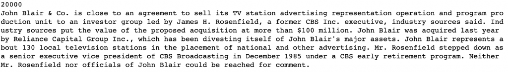
在NLTK上有許多手動進行詞性標注的文集了。本次使用Penn Treebank文集(the Penn Treebank Corpus)以及Brown文集(the Brown Corpus)。其中Penn Treebank中搜集了許多華爾街日報的文章(Wall Street Journal),而Brown中多數的文字和文學有關。在以下這格中我們下載Penn Treebank以及Brown這兩個文集,並且測試了這兩個文集中的第一個句子。".tagged_sents()"提取了詞性標註過的句子(sents = sentences)。
import nltk
from nltk.corpus import treebank, brown
nltk.download('treebank')
nltk.download('brown')
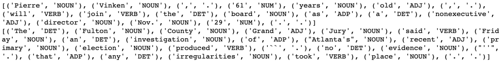
print(treebank.tagged_sents()[0])
print(brown.tagged_sents()[0])
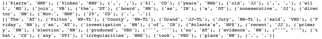
在NLTK中,文字和標註的組合是以tuple的方式儲存的。然而在實作上,詞性標註常以"word/tag"的方式顯示,例如"Pierre/NNP", "the/DT"。NNP是指專有名詞、DT則為定冠詞,完整的標籤列表大家可以參考:https://www.ling.upenn.edu/courses/Fall_2003/ling001/penn_treebank_pos.html 。
值得注意的是,這兩個文集並不是使用相同的標註方式。同樣是"the",Brown把它標註成"AT"(Article,冠詞),而在Penn Treebank中則被標註為"DT(Determiner,定冠詞)。好消息是,在NLTK中也可以把他們都轉換成Universal標註方式。https://universaldependencies.org/u/pos/ 。
import nltk
nltk.download('universal_tagset')
print(treebank.tagged_sents(tagset="universal")[0])
print(brown.tagged_sents(tagset="universal")[0])
知道詞性標註的基本規則之後,開始開發一個Unigram Tagger。首先,我們需要先記錄每一個字形是出現各種詞性的頻率。我們可以將它存在python資料結構的dict中dict(事實上這不是最有效率的存法 :D)。雖然前面也介紹Brown Corpus,但從這邊開始我們專注於使用Penn Treebank的標籤規則。
from collections import defaultdict

POS_dict = defaultdict(dict)
for word_pos_pair in treebank.tagged_words():
    word = word_pos_pair[0].lower() # 正規化成小寫
    POS = word_pos_pair[1]
    POS_dict[word][POS] = POS_dict[word].get(POS,0) + 1
取一些字來看看他們怎麼表現多個詞性標註,以及每個詞性在文集中的分布狀況:
for word in list(POS_dict.keys())[900:1000]:
    if len(POS_dict[word]) > 1:
        print(word)
        print(POS_dict[word])
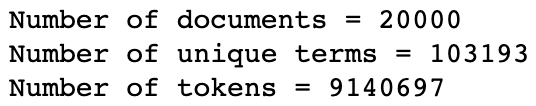
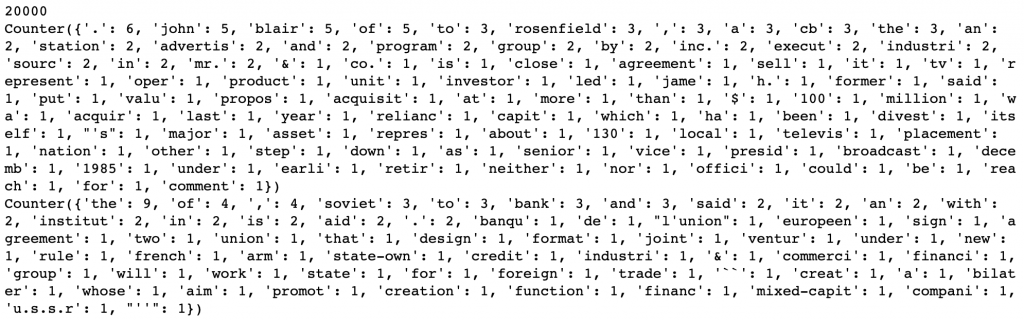
結果會如同這張圖所顯示:
觀察到一些常見的歧義會發生在名詞和動詞之間(plans, decline, cost);在動詞之間,過去式和過去分詞也會發生同樣的問題(announced, offered, spent).
為了開發出第一個標註器(Unigram Tagger),只需要為每個詞選出最常見的詞性。
tagger_dict = {}
for word in POS_dict:
tagger_dict[word] = max(POS_dict[word],key=lambda x: POS_dict[word][x])
def tag(sentence):
return [(word,tagger_dict.get(word,"NN")) for word in sentence]
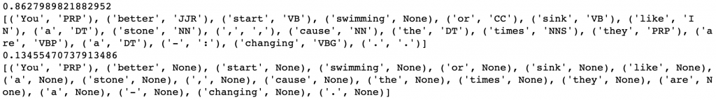
example_sentence = """You better start swimming or sink like a stone , cause the times they are a - changing .""".split()
print(tag(example_sentence))

因為不是每一個字都是在training set中看過的字,所以遇到沒有看過的字,會自動標註成名詞"NN"。我們可以觀察到這樣的方法雖然會有一些問題,例如"swimming"在該是動詞,卻因此被標註成了名詞。然而總體而言,這樣標註的成效還挺不錯的。
NLTK也有內建的N-gram tagger,可以使用內建的Unigram(1-gram)和Bigram(2-gram) Tagger。
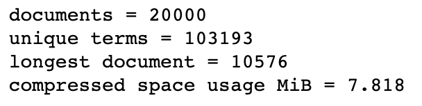
首先,需要將文集切割成訓練集和測試集。
# 訓練集:測試集 = 9:1
size = int(len(treebank.tagged_sents()) * 0.9)
train_sents = treebank.tagged_sents()[:size]
test_sents = treebank.tagged_sents()[size:]
先來比對預設的Unigram和Bigram Tagger。NLTK裡面所有的標註器都有評價功能,藉此回傳測試集運行在這個訓練模型的準確率(accuracy)。
from nltk import UnigramTagger, BigramTagger

unigram_tagger = UnigramTagger(train_sents)
bigram_tagger = BigramTagger(train_sents)
print(unigram_tagger.evaluate(test_sents))
print(unigram_tagger.tag(example_sentence))
print(bigram_tagger.evaluate(test_sents))
print(bigram_tagger.tag(example_sentence))
在這裡Unigram Tagger的效果好太多了。原因很明顯,因為Bigram Tagger並沒有足夠的資料來觀察前後文的關係;更糟的是,一旦一個詞的詞性判斷被判定成"None",後面整句話也都會失敗。
為了解決問題,需要為Bigram Tagger加上退避(backoffs)。關於backoffs,這是關於N-gram語言模型和Smoothing的問題,目前先不說明,現在就先預設那些"None"的字為"NN"。
from nltk import DefaultTagger

default_tagger = DefaultTagger("NN")
unigram_tagger = UnigramTagger(train_sents,backoff=default_tagger)
bigram_tagger = BigramTagger(train_sents,backoff=unigram_tagger)

print(bigram_tagger.evaluate(test_sents))
print(bigram_tagger.tag(example_sentence))

藉由退避方法,我們將Bigram的資訊加到Unigram之上,準確率也有了3%的提升。

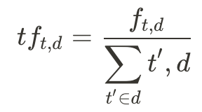
 ,其中
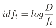
,其中